Annotations in Object Detection: Transforming XY coordinates into COCO format
Written on October 16th, 2023 by Alvaro Carranza
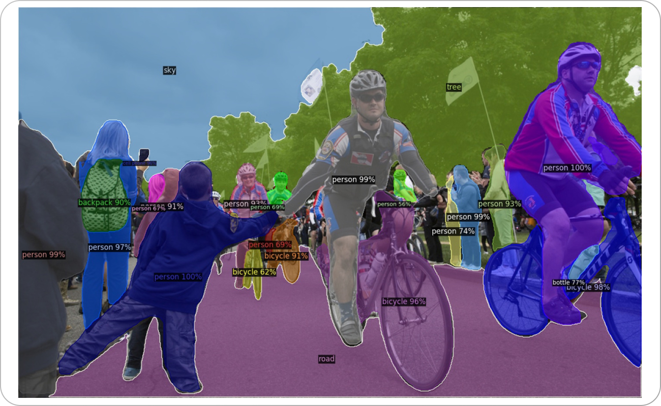
Image from COCO dataset (source)
Data is often messy or incomplete. For this reason, data preprocessing (which includes labeling) is one of the most important steps in data analysis and data science.
During the first stages of HS Detector Web App, a tool I developed - alongside 4 other students - for early detection of Hereditary Spherocytosis (an inherited blood disorder that happens when red blood cells (RBCs from now on) are shaped like a sphere instead of a disk, named spherocytes), we settled on using two datasets to train a Deep Learning model for object detection (a classification and localization task, of RBCs in this case):
- Dataset A: a dataset of 186 digital images of RBC blood smears from five patients with hereditary spherocytosis;
- Chula-RBC-12-Dataset: a dataset of RBC blood smear images used in “Red Blood Cell Segmentation with Overlapping Cell Separation and Classification from an Imbalanced Dataset” (2023), containing 12 classes of RBC types consisting of 706 smear images that contain over 20,000 RBCs.
Image annotation (labeling digital images) is a central part of training computer vision models that process image data for object detection, classification, segmentation and more. For instance, bounding boxes can be placed around objects to label each type or category.
Bounding boxes applied to identify vehicle types and pedestrians (source)
While we used Roboflow’s Model-Assisted Labeling to quickly annotate Dataset A, the Chula-RBC-12-Dataset annotation would be a much more difficult task considering it included 12 classes (in this case RBC types).
Its repository includes a “Label” folder that contains label data in a specific way. You can find .txt files inside with the name of the corresponding image, each file containing multiple lines (one for each RBC label). Each line is stored in the following sequence:
- x coordinate;
- y coordinate;
- type of RBC in number (0 for a normal RBC, 1 for a macrocyte, 2 for a microcyte, 3 for a spherocyte…)
However, Roboflow’s output was in COCO format, a JSON structure that governs how labels and metadata are formatted for a dataset. This format originates from Microsoft’s Common Objects in Context dataset (COCO), one of the most popular object detection datasets (you can find more information on COCO in this paper). Correctly annotating Chula-RBC-12-Dataset in the same format as the Rofoflow’s output (COCO format) was vital to use both datasets in future developments (e.g. detecting other RBC types and thus other diseases).
I digged deeper into the documentation of this format and decided to write a utility function in Python to transform the label data provided with the Chula-RBC-12-Dataset in .txt files (essentially XY coordinates and a label type) into COCO format.
import os
import json

# Parse the TXT files and associate annotations with images
annotations = []
images = []

label_folder = # Same folder as "Label" repository's folder
dataset_folder = # Same folder as "Dataset" repository's folder

for txt_file in os.listdir(label_folder):
    if txt_file.endswith(".txt"):
        image_id = int(os.path.splitext(txt_file)[0])
        image_filename = f"{image_id}.jpg"
        image_path = os.path.join(dataset_folder, image_filename)

        # Check if the corresponding image exists
        if os.path.exists(image_path):
            with open(os.path.join(label_folder, txt_file), 'r') as txt_file:
                annotation_id = 1
                for line in txt_file:
                    # a and b are xy coord of the center of the annotation
                    a, b, category = map(int, line.strip().split())
                    # s is an arbitrary size to fit all RBCs
                    s = 70
                    x_min = a - (s/2)
                    x_max = a + (s/2)
                    y_min = b - (s/2)
                    y_max = b + (s/2)
                    annotation = {
                        "id": annotation_id,
                        "image_id": image_id,
                        "category_id": category,
                        # bbox that should account for most RBCs
                        "bbox": [x_min, y_min , s, s],
                        # area calculation for a square bbox
                        "area": s*s,
                        # segmentation calculation with xs and ys
                        "segmentation": [x_min,
                                          y_min,
                                          x_min,
                                          y_min + y_max,
                                          x_min + x_max,
                                          y_min + y_max,
                                          x_min + x_max,
                                          y_max
                                          ],
                        "iscrowd": 0  # 0 for individual annotation
                    }
                    annotations.append(annotation)
                    annotation_id += 1

            images.append({
                "id": image_id,
                "file_name": image_filename
            })

# Create a list with corresponding id_names
id_names = {0: "RBC",
            1: "Macrocyte",
            2: "Microcyte",
            3: "Spherocyte",
            4: "Target cell",
            5: "Stomatocyte",
            6: "Ovalocyte",
            7: "Teardrop",
            8: "Burr cell",
            9: "Schistocyte",
            10: "uncategorised",
            11: "Hyochromia",
            12: "Elliptocyte"
            }

# Create the COCO annotation data structure
coco_data = {
    "info": {"year": 2023,
            "version": "1",
            "description": "Chula-RBC-12-Dataset COCO annotations",
            "contributor": "",
            "url": "",
            "date_created": "2023"
            },
    "licenses": [],
    "images": images,
    "categories": [
        {
            "id": category,
            "name": id_names[category],
            # Assign all to the "Blood smear images" supercategory
            "supercategory": "Blood smear images"
        }
        for category in set(annotation["category_id"] for annotation in annotations)
    ],
    "annotations": annotations
}

# Write the COCO data to a JSON file
with open("chula_coco_annotations.json", "w") as json_file:
    json.dump(coco_data, json_file)
Some extra comments:
- I discovered not all images had label data, so I also had to take that into account (only 623 out of +700 images had the corresponding label data);
- As I only had XY coordinates to begin with, I had to make some compromises and have a standard size for bounding boxes (all squares of “s” width and height) that could fit all RBCs;
- Additional information to create the utility function - specially how to calculate segmentation - was found on “Understanding COCO Dataset” article by Srishiles P S
- Even if not used in the current deployment, you can find the actual function in HS Detector Web App’s repository.
Although quite simple, finding a solution to this formatting problem allowed me to:
- Put my Python skills to the test;
- Demistify JSON, the go-to format for exchanging data between web servers and clients;
- Better understand the COCO Dataset;
- Highlight the importance of image annotation in computer vision models.

